class: center, middle, inverse, title-slide .title[ # Tests for Association ] .subtitle[ ## Pearson’s, Spearman’s and Kendall’s ] .author[ ### Jyotishka Datta ] .date[ ### Updated: 2023-11-07 ] --- ## Pearson's Correlation Coefficient Let's look at the "cars" data available on R. ```r library(MASS) attach(cars) head(cars) ``` ``` ## speed dist ## 1 4 2 ## 2 4 10 ## 3 7 4 ## 4 7 22 ## 5 8 16 ## 6 9 10 ``` --- ## Scatter plot The scatter plot has an upward trend indicating positive trend! <!-- --> --- ## Best fit line We can try to fit a straight line or a curve to the scatter plot. The best-fitting curve looks somewhat linear and shows an upward trend. 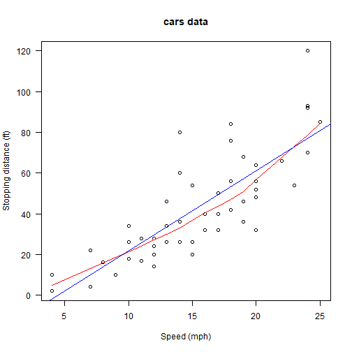<!-- --> --- ## Correlation The R functions you need are `cor` and `cor.test`. The latter does the `\(t\)`-test for testing `\(H_0: \rho = 0\)`. ```r cor(cars$speed,cars$dist) ``` ``` ## [1] 0.8068949 ``` ```r cor.test(cars$speed,cars$dist) ``` ``` ## ## Pearson's product-moment correlation ## ## data: cars$speed and cars$dist ## t = 9.464, df = 48, p-value = 1.49e-12 ## alternative hypothesis: true correlation is not equal to 0 ## 95 percent confidence interval: ## 0.6816422 0.8862036 ## sample estimates: ## cor ## 0.8068949 ``` --- ## Log transform? ```r plot(cars, xlab = "Speed (mph)", ylab = "Stopping distance (ft)", las = 1, log = "xy") title(main = "cars data (logarithmic scales)") ``` 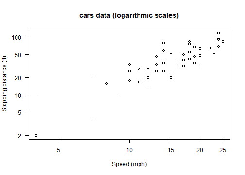<!-- --> --- ## Does the correlation improve? ```r cor(log(cars$speed),log(cars$dist)) ``` ``` ## [1] 0.8562385 ``` ```r cor.test(log(cars$speed),log(cars$dist)) ``` ``` ## ## Pearson's product-moment correlation ## ## data: log(cars$speed) and log(cars$dist) ## t = 11.484, df = 48, p-value = 2.259e-15 ## alternative hypothesis: true correlation is not equal to 0 ## 95 percent confidence interval: ## 0.7587175 0.9162214 ## sample estimates: ## cor ## 0.8562385 ``` --- ## Remember the properties 1. `\(X\)` and `\(Y\)` independent `\(\Rightarrow\)` `\(\rho_{X,Y} = 0\)`, but not the other way round, unless `\(X,Y\)` are jointly normal. 2. Correlation is always between -1 and +1, with the extreme values indicating perfect linear relationship. 3. Correlation `\(\not \Rightarrow\)` Causation. There could be a **lurking** variable, causing a **spurious** relationship. 4. Lots of hilarious examples in [Spurious Correlations Webpage](http://tylervigen.com/spurious-correlations) --- ## Example - Here `\(\rho_{X,Y} = 0\)`, but `\(Y = X^2\)`, not independent, but not **linearly dependent**. ```r x = c(-5,-4,-3,-2,-1,1,2,3,4,5);y = x^2 cor(x,y) ``` ``` ## [1] 0 ``` <img src="association_demo_files/figure-html/unnamed-chunk-8-1.png" style="display: block; margin: auto;" /> --- class: inverse, center, middle # Spearman's correlation --- ## Motivation - Pearson's correlation coefficient measures only linear relationship. Here `\(y = x^4\)`: a perfect montonically increasing relationship but the Pearson's correlation is still not 1. ```r x = seq(1,7) y = x^4 cor(x,y) ``` ``` ## [1] 0.8903055 ``` ```r ## same as cor(x,y,method="pearson") cor(x,y,method="pearson") ``` ``` ## [1] 0.8903055 ``` --- ## Spearman's rank correlation - Spearman's rank correlation: replace X, Y with their ranks. ```r cor(rank(x),rank(y)) ``` ``` ## [1] 1 ``` ```r ## same as cor(x,y,method="spearman") cor(x,y,method="spearman") ``` ``` ## [1] 1 ``` - Spearman's `\(r_s\)` measure monotonic association. `\(r_s = 1\)` means X is a monotonically increasing function of Y. --- ## Transformation invariance - Spearman's `\(r_s\)` is preserved if we apply the same monotone order-preserving transformation to both `\(X\)` and `\(Y\)`. - Example: Apply log transformation to cars data, Pearson's r will change, but Spearman's `\(r_s\)` won't! ```r cor(cars$speed,cars$dist) ``` ``` ## [1] 0.8068949 ``` ```r cor(log(cars$speed),log(cars$dist)) ``` ``` ## [1] 0.8562385 ``` --- ## Spearman's rank correlation - As long as the transformation is monotone: `\(f(x) = log(x)\)`, `\(f(x) = x^2\)`. ```r cor(cars$speed,cars$dist,method="spearman") ``` ``` ## [1] 0.8303568 ``` ```r cor(log(cars$speed),log(cars$dist),method="spearman") ``` ``` ## [1] 0.8303568 ``` ```r cor((cars$speed)^2,(cars$dist)^2,method="spearman") ``` ``` ## [1] 0.8303568 ``` --- ## Hypothesis test ```r cor.test(cars$speed,cars$dist,method="spearman") ``` ``` ## Warning in cor.test.default(cars$speed, cars$dist, method = "spearman"): Cannot ## compute exact p-value with ties ``` ``` ## ## Spearman's rank correlation rho ## ## data: cars$speed and cars$dist ## S = 3532.8, p-value = 8.825e-14 ## alternative hypothesis: true rho is not equal to 0 ## sample estimates: ## rho ## 0.8303568 ``` --- ## Kendall's tau - Kendall's tau measures the association by measuring concordance or discordance in the data. - If `\(p_c\)` and `\(p_d\)` denote the probability of concordance and discordance respectively: then Kendall's coefficient `\(\tau\)` is defined as: $$ \tau = p_c - p_d $$ - Since `\(p_c + p_d = 1\)`, you can also write `\(\tau\)` in terms of only `\(p_c\)` or `\(p_d\)`. --- ## Kendall's tau Kendall's tau is related to Pearson's product-moment correlation coefficient as: $$ \tau = \frac{2}{\pi} \arcsin(\rho) $$ - Here's the functional relationship. <!-- --> --- ## Kendall's tau ```r cor(cars$speed,cars$dist,method="kendall") ``` ``` ## [1] 0.6689901 ``` ```r cor(log(cars$speed),log(cars$dist),method="kendall") ``` ``` ## [1] 0.6689901 ``` ```r cor((cars$speed)^2,(cars$dist)^2,method="kendall") ``` ``` ## [1] 0.6689901 ``` --- ## In class example ```r x = c(1, 5, 9, 7, 4, 6, 8, 2, 3) y = c(4, 3, 6, 8, 2, 7, 9, 1, 5) cor(x,y, method = "spearman") ``` ``` ## [1] 0.7166667 ``` ```r cor.test(x,y, method = "spearman") ``` ``` ## ## Spearman's rank correlation rho ## ## data: x and y ## S = 34, p-value = 0.03687 ## alternative hypothesis: true rho is not equal to 0 ## sample estimates: ## rho ## 0.7166667 ``` --- ## In class example How good is the normal approximation? ```r x = c(1,5,9,7,4,6,8,2,3) y = c(4,3,6,8,2,7,9,1,5) n = length(x) r_s = cor(x,y, method = "spearman") (normal.p.value = 2*(1 - pnorm(sqrt(length(x)-1)*r_s))) ``` ``` ## [1] 0.04265838 ``` ```r (t.p.value = 2*(1 - pt((r_s*sqrt(n-2))/sqrt(1-r_s^2),df = n-2))) ``` ``` ## [1] 0.02981804 ``` - The exact P-value is 0.03687. Which one is closer? --- ## In class example ```r x = c(1, 5, 9, 7, 4, 6, 8, 2, 3) y = c(4, 3, 6, 8, 2, 7, 9, 1, 5) cor.test(x,y, method = "kendall") ``` ``` ## ## Kendall's rank correlation tau ## ## data: x and y ## T = 28, p-value = 0.04462 ## alternative hypothesis: true tau is not equal to 0 ## sample estimates: ## tau ## 0.5555556 ``` --- ## In class example Using the Normal approximation: $$ Z = 3 \sqrt{n(n-1)}\tau/\sqrt{2(2n+5)} $$ ```r x = c(1,5,9,7,4,6,8,2,3) y = c(4,3,6,8,2,7,9,1,5) n = length(x) T = cor(x,y, method = "kendall") Z = 3*sqrt(n*(n-1))*T/sqrt(2*(2*n+5)) normal.p.value = 2*(1 - pnorm(Z)) cat("P value = ", normal.p.value, "\n") ``` ``` ## P value = 0.03705622 ``` - Exact P-value = 0.04462. (See last slide.) --- ## Divorce Example - Mann's Test (Kendall's) ```r year = seq(1945,1985,by=5) divorce.rate = c(3.5, 2.6, 2.3, 2.2, 2.5, 3.6, 4.8, 5.2, 5) cor.test(year,divorce.rate, method = "kendall") ``` ``` ## ## Kendall's rank correlation tau ## ## data: year and divorce.rate ## T = 27, p-value = 0.07518 ## alternative hypothesis: true tau is not equal to 0 ## sample estimates: ## tau ## 0.5 ``` --- ## Divorce Example - Daniel's Test (Spearman's) ```r year = seq(1945,1985,by=5) divorce.rate = c(3.5, 2.6, 2.3, 2.2, 2.5, 3.6, 4.8, 5.2, 5) cor.test(year,divorce.rate, method = "spearman") ``` ``` ## ## Spearman's rank correlation rho ## ## data: year and divorce.rate ## S = 36, p-value = 0.04325 ## alternative hypothesis: true rho is not equal to 0 ## sample estimates: ## rho ## 0.7 ```