Quantile Importance Sampling
Multivariate t

rm(list = ls())
# Set global R options
options(scipen = 4)

# Set the graphical theme
ggplot2::theme_set(ggplot2::theme_light())

# Set global knitr chunk options
knitr::opts_chunk$set(
  warning = FALSE, 
  message = FALSE,
  cache = TRUE
)

set.seed(123)

library(truncnorm)
library(pracma)
library(ggplot2)

Multivariate \(t\) Example

As an example of a higher-dimensional integral, we look at a multivariate \(t\) likelihood and a multivariate Gaussian prior with dimension \(d = 50\), following Polson and Scott (2014). The target integral is:

\[ Z = \int_{\mathbb{R}^d} (1 + \frac{x^T x}{\nu})^{-\frac{\nu + d}{2}} (\frac{\tau}{2\pi})^{d/2} \exp \{-\tau x^T x / 2\} d x. \]

This integral can be written in terms of Kummer’s confluent hypergeometric function of the second kind: \(Z = s^{a}U(a, b, s)\), where \(a = (\nu + d)/2\), \(b = \nu/2 + 1\), \(s = \nu \tau/2\). For the specific values used here: \(d = 50, \tau =1\) and \(\nu = 2\), we can get: \(Z = U(26, 2, 1) = 1.95\times 10^{-29}\).

We show the R codes for comparing QIS with naive Monte Carlo.

Estimation by QIS, and Naive MC

We define three essential functions below:

• vertical.grid will generate an \(x\)-grid for integration using either the exponential weights (for original nested sampling), or uniform for Yakowitz (Quantile Importance Sampling. )
• sQ is simply a sample quantile calculator.

# Generate grid
vertical.grid = function(l,N,type = NULL){
  # "u" - uniform
  # "e" - exponential
  
  if(type == "u"){
    ugrid = runif(N)
    res = c(sort(ugrid),1)
    # res = sort(runif(N))
  }else if(type == "e"){
    res = exp(-(0:l)/N)
  }
  
  return(res)
}
# Quantile
sQ = function(q,Y){
  # q-quantile of Y
  N = length(Y)
  res = Y[ceiling(N*q)]
  return(res)
}

Naive Monte Carlo

# Test example
# Prior and Likelihood

set.seed(90210)

d = 50
tau = 1
nu = 2

trueZ <- 1.9445572*10^(-29) ## U(26,2,1), d = 50, nu = 2, s = 1

dtmvr <- function(x, nu){
  d = length(x)
  logden = -0.5*(nu + d)*log(1 + (t(x)%*%x)/nu)
  return(exp(logden))
}

library(LaplacesDemon)


r = 100

mc.naive = NULL
verbose = TRUE
for(i in 1:r){
  if(isTRUE(verbose) && i %% 10 == 0)
    cat("Iteration ",i, "\n")
  M = 10000
  # X = rmvn(M, rep(0,d), eye(d))
  Y = numeric(M)
  for(j in 1:M){
    Y[j] = dtmvr(x = rnorm(d, 0, 1), nu = 2)
  }
  mc.naive = c(mc.naive,mean(Y))
}

Iteration  10 
Iteration  20 
Iteration  30 
Iteration  40 
Iteration  50 
Iteration  60 
Iteration  70 
Iteration  80 
Iteration  90 
Iteration  100 

mean(mc.naive)

[1] 4.538692e-31

summary(mc.naive)

     Min.   1st Qu.    Median      Mean   3rd Qu.      Max. 
7.554e-33 3.820e-32 7.599e-32 4.539e-31 1.793e-31 2.362e-29 

Quantile Importance Sampling

set.seed(90210)

## QIS 

N = 20
# r = 100

mc.qis = NULL
verbose = TRUE

simu.grid.unif = vertical.grid(l=NULL,N,type = "u")

for(i in 1:r){
  
  if(isTRUE(verbose) && i %% 10 == 0)
    cat("Iteration ",i, "\n")
  M = 10000
  # X = rmvn(M,rep(0,d), eye(d))
  Y = numeric(M)
  for(j in 1:M){
    Y[j] = dtmvr(x = rnorm(d, 0, 1), nu = 2)
  }
  Y = sort(Y)
  Lambda = sQ(simu.grid.unif,Y)
  
  x = simu.grid.unif
  y = Lambda
  # Use a correction term at the boundary: -h^2/12*(f'(b)-f'(a))
  # h  <- x[2] - x[1]
  # ca <- (y[2]-y[1]) / h
  # cb <- (y[N]-y[N-1]) / h
  # YakoMC <- trapz(x, y) - h^2/12 * (cb - ca)
  YakoMC <- trapz(x, y)
  
  # mc.qis = c(mc.qis, trapz(simu.grid.unif,Lambda)) ## QIS Original 
  mc.qis = c(mc.qis, YakoMC) ## QIS Corrected
}

Iteration  10 
Iteration  20 
Iteration  30 
Iteration  40 
Iteration  50 
Iteration  60 
Iteration  70 
Iteration  80 
Iteration  90 
Iteration  100 

## Trim top and bottom 2.5%

trim_ul <- function(x, p = 0.01){
   x <- x[x >= quantile(x, p) & x <= quantile(x, 1-p)]
   return(x)
}
  
cbind(mean(trim_ul(mc.qis, p = 0.025)), mean(trim_ul(mc.naive, p = 0.025)), trueZ)

                                      trueZ
[1,] 7.845875e-29 1.820323e-31 1.944557e-29

Comparison

Graphically, …

library(ggplot2)
mc.data = rbind(data.frame(MC = trim_ul(mc.qis, p = 0.025), method = "QIS"),
                data.frame(MC = trim_ul(mc.naive, p = 0.025), method = "Naive MC"))

(plt <- ggplot(mc.data, aes(MC, fill = method)) + 
    geom_histogram(alpha=0.75, bins = 30, position="identity",aes(y = after_stat(density)))+
    geom_density(alpha=0.75, stat="density",position="identity",aes(y = after_stat(density)))+
    expand_limits(x = c(1e-33,1e-25))+
        geom_vline(xintercept=trueZ)+scale_x_log10()+
    # coord_flip()+ 
    facet_wrap(vars(method), ncol = 1, scales = "free_y")+
    theme_minimal()+
    labs(title = "QIS vs. Naive MC", subtitle = "Multivariate t, MVN prior"))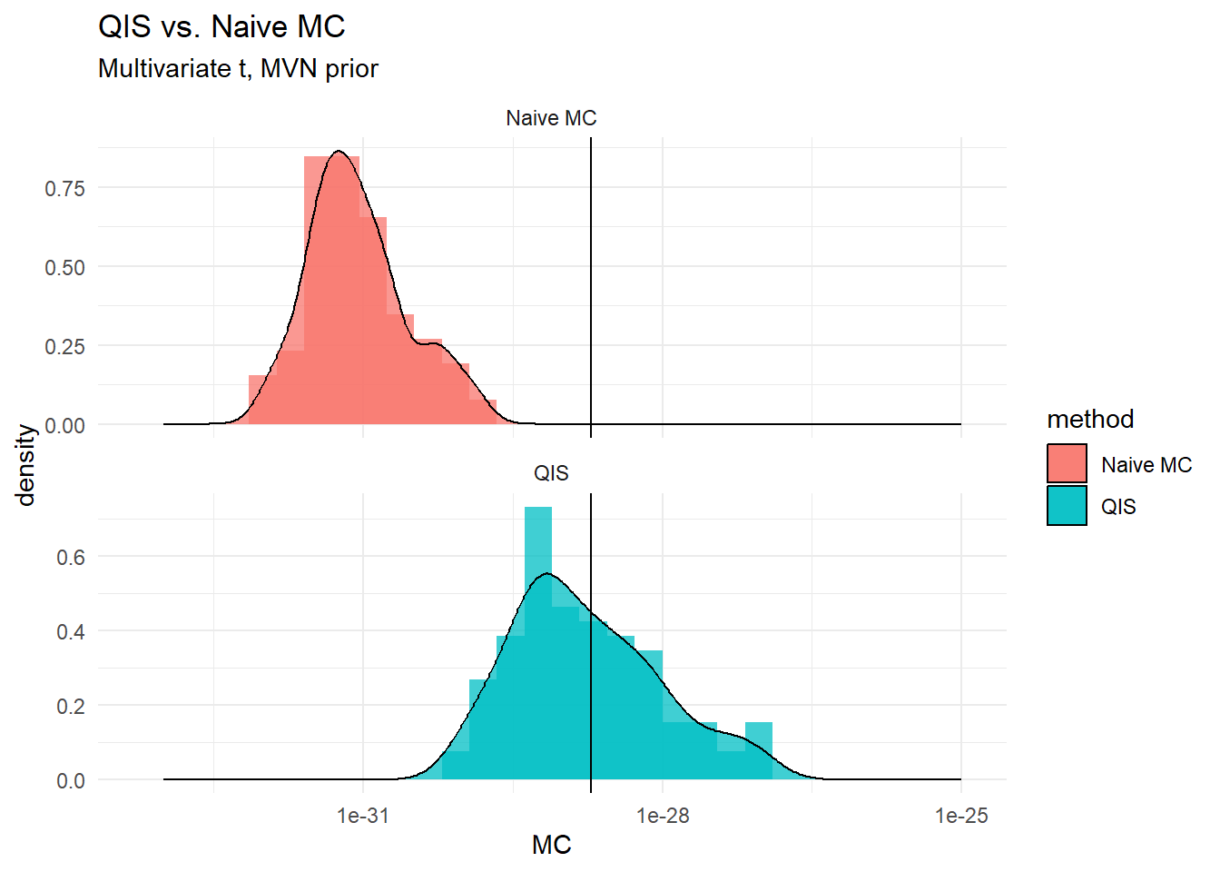

Numerically, …

## Numerical 

mean.qis <- mean(mc.qis, trim = 0.025); mean.naive <- mean(mc.naive,trim = 0.025)
median.qis <- median(mc.qis); median.naive <- median(mc.naive)
mape.qis <- median(abs((mc.qis)-(trueZ))/(trueZ))
mape.naive <- median(abs(((mc.naive)-(trueZ))/(trueZ)))
rmse.qis <- sqrt((mean((mc.qis-trueZ)^2)))
rmse.naive <- sqrt((mean((mc.naive-trueZ)^2)))

perf <- rbind((cbind(mean.qis,mean.naive)),
              (cbind(median.qis,median.naive)),
              (cbind(mape.qis, mape.naive)),
              (cbind(rmse.qis,rmse.naive)))

colnames(perf) <- c("QIS", "Naive"); row.names(perf) <- c("Mean", "Median",
                                                          "MAPE", "RMSE")
library(knitr)
library(kableExtra)

kable(perf, format = "html", digits = 99)  %>%
  kable_styling()

	QIS	Naive
Mean	8.672069e-29	2.007210e-31
Median	1.376328e-29	7.598928e-32
MAPE	8.243520e-01	9.960922e-01
RMSE	3.994507e-28	1.913807e-29