Quantile Importance Sampling
Normal-Normal

rm(list = ls())
# Set global R options
options(scipen = 999)

# Set the graphical theme
ggplot2::theme_set(ggplot2::theme_light())

# Set global knitr chunk options
knitr::opts_chunk$set(
  warning = FALSE, 
  message = FALSE,
  cache = TRUE
)

set.seed(12345)

library(truncnorm)
library(pracma)
library(ggplot2)

Example

We take Gaussian likelihood and Gaussian prior,

\[ \begin{align*} L(x \mid \mu_1, \sigma_1) & = \frac{1}{\sqrt{2 \pi}\sigma_1} e^{-\frac{(x-\mu_1)^2}{2\sigma_1^2}},\\ p(x \mid \mu_2, \sigma_2) & = \frac{1}{\sqrt{2 \pi}\sigma_2} e^{-\frac{(x-\mu_2)^2}{2\sigma_2^2}} \end{align*} \]

The integral \(Z = \int L(x) p(x) dx\) is available in closed form due to the self-conjugacy property of Gaussian prior with the mean parameter of a Gaussian distribution. To see this, note that we can write the product of two Gaussian density functions in the following way:

\[ \begin{gather} \phi(x \mid \mu_1, \sigma_1) \times \phi(x \mid \mu_2, \sigma_2) = \phi(\mu_1 \mid \mu_2, \sqrt{\sigma_1^2 + \sigma_2^2}) \times \phi(x \mid \mu_{\text{post}}, \sigma_{\text{post}}^2) \\ \text{where} \quad \mu_{\text{post}} = \frac{\sigma_1^{-2} \mu_1 + \sigma_2^{-2} \mu_2}{\sigma_1^{-2} + \sigma_2^{-2}}, \sigma_{\text{post}}^2 = \frac{\sigma_1^2 \sigma_2^2}{\sigma_1^2 + \sigma_2^2}. \end{gather} \]

Integrating the right-hand-side will leave the normalizing constant, here expressed as a Gaussian density itself. Let \(\mu_1 = 2, \mu_2 =0\) and \(\sigma_1^2 = \sigma_2^2 = 1\). The normalizing constant will be:

\[ Z = \phi(2 \mid 0, 2) = \frac{1}{\sqrt{2 \pi} \sqrt{2}} e^{-1} = \frac{1}{2 e \sqrt{\pi}}. \]

Estimation by QIS, NS and Naive MC

We define three essential functions below:

• vertical.grid will generate an \(x\)-grid for integration using either the exponential weights (for original nested sampling), or uniform for Yakowitz (Quantile Importance Sampling. )
• sQ is simply a sample quantile calculator.
• nested_sampling performs the nested sampling algorithm: removes the lowest likelihood, simulates a new draw from the constrained prior space and calculates the Lorenz curve.

# Generate grid
vertical.grid = function(l,N,type = NULL){
  # "u" - uniform
  # "e" - exponential
  
  if(type == "u"){
    ugrid = runif(N)
    res = c(sort(ugrid),1)
    # res = sort(runif(N))
  }else if(type == "e"){
    res = exp(-(0:l)/N)
  }
  
  return(res)
}
# Quantile
sQ = function(q,Y){
  # q-quantile of Y
  N = length(Y)
  res = Y[ceiling(N*q)]
  return(res)
}
# Nested sampling (normal prior, normal likelihood)
nested_sampling = function(mu1,sigma1,mu2,sigma2,N,tol=0.001){
  # "mu1", "sigma1" - likelihood
  # "mu2", "sigma2" - prior
  
  Lmax = 1/(sqrt(2*pi)*sigma1)
  
  theta = rnorm(N,mu2,sigma2)
  L = dnorm(theta,mu1,sigma1)
  phi = NULL
  error = 1
  
  while(error >= tol)
  {
    index = which.min(L)
    Lmin = min(L)
    phi = c(phi,Lmin)
    
    error = abs(Lmin-Lmax)/Lmax
    
    term = -log(Lmin*sqrt(2*pi)*sigma1)
    a = mu1 - sqrt(term*2*sigma1^2) 
    b = mu1 + sqrt(term*2*sigma1^2)
    
    newTheta = rtruncnorm(1,a,b,mean = mu2,sd = sigma2)
    newL = dnorm(newTheta,mu1,sigma1)
    theta[index] = newTheta
    L[index] = newL
  }
  return(list(phi=phi, L = L))
}

Naive Monte Carlo

# Test example
# Prior and Likelihood
mu1 = 2
sigma1 = 1
mu2 = 0
sigma2 = 1 

(trueZ = 1/(2*exp(1)*sqrt(pi)))

[1] 0.1037769

N = 100
r = 1000
mc.naive = NULL
verbose = FALSE
for(i in 1:r){
  if(isTRUE(verbose) && i %% 100 == 0)
    cat("Iteration ",i, "\n")
  X = rnorm(N,mu2,sigma2)
  Y = dnorm(X,mu1,sigma1) 
  mc.naive = c(mc.naive,sum(Y)/N)
}

mean(mc.naive)

[1] 0.1038586

hist(mc.naive, breaks = 30, main = "Naive Monte Carlo Estimates")
abline(v=trueZ,col="red",lwd=2)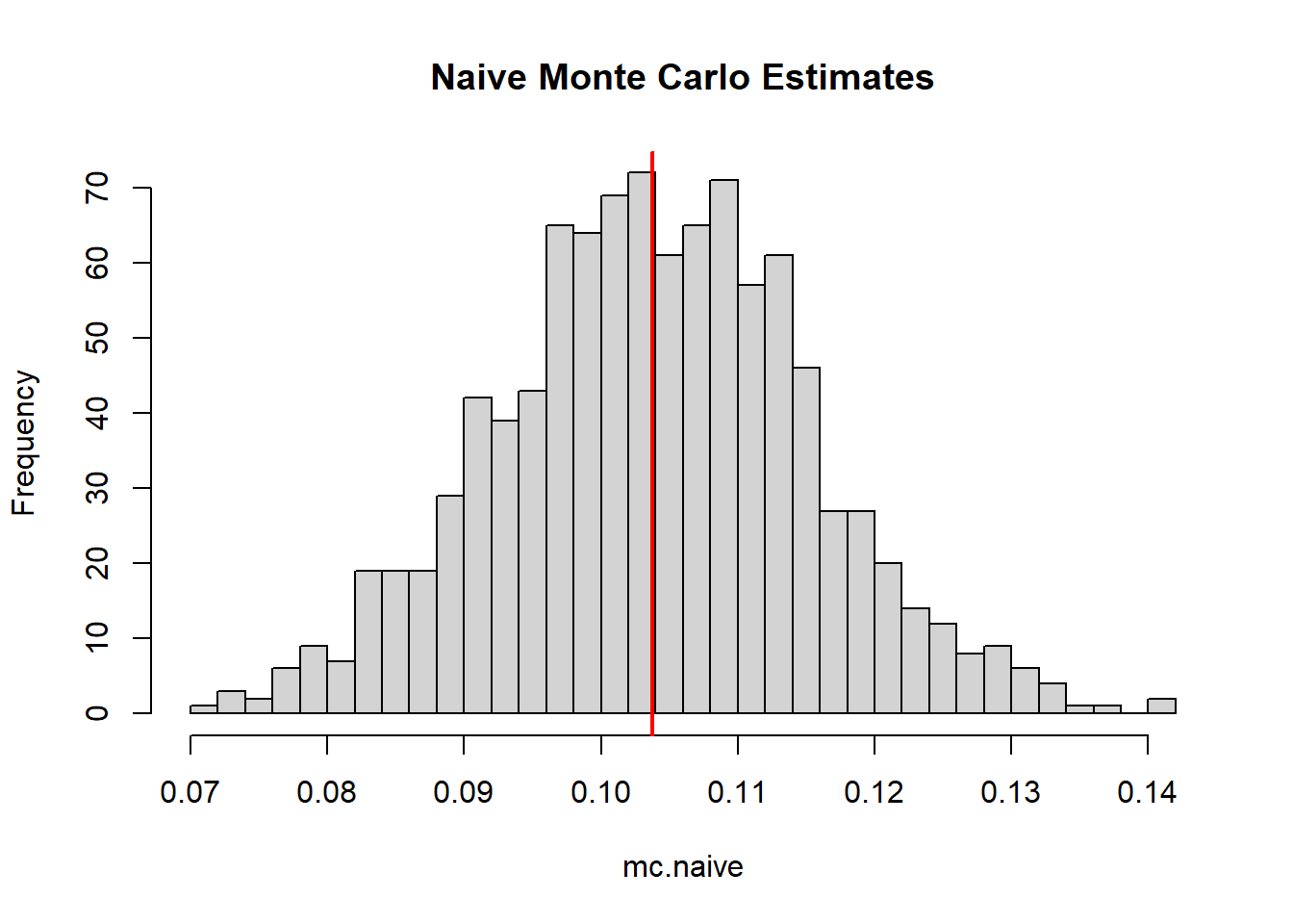

Quantile Importance Sampling

N = 100
r = 1000

mc.qis = NULL
verbose = FALSE


for(i in 1:r){
  
  if(isTRUE(verbose) && i %% 10 == 0)
    cat("Iteration ",i, "\n")
  M = 1000
  X = rnorm(M,mu2,sigma2)
  Y = dnorm(X,mu1,sigma1) 
  Y = sort(Y)
  
  simu.grid.unif = vertical.grid(l=NULL,N,type = "u")

  Lambda = sQ(simu.grid.unif,Y)
  mc.qis = c(mc.qis,trapz(simu.grid.unif,Lambda)) ## QIS 
}

mean(mc.qis)

[1] 0.103908

hist(mc.qis, breaks = 30, main = "QIS (Yakowitz) Estimates")
abline(v=trueZ,col="red",lwd=2)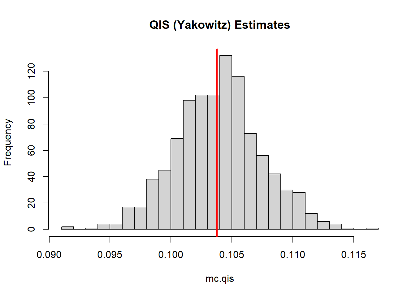

Nested Sampling with exponential weights

mc.nested = NULL
mc.nested.rect = NULL
verbose = FALSE


for(i in 1:r){
  
  if(isTRUE(verbose) && i %% 10 == 0)
    cat("Iteration ",i, "\n")
  M = 1000
  X = rnorm(M,mu2,sigma2)
  Y = dnorm(X,mu1,sigma1) 
  Y = sort(Y)
  
  value = nested_sampling(mu1,sigma1,mu2,sigma2,N,tol = 1e-7)
  simu.grid = vertical.grid(length(value$phi),N,"e")
  
  # Lambda = sQ(simu.grid,Y)
  mc.nested = c(mc.nested,-trapz(simu.grid[-1],value$phi)) ## Trapezoidal rule (Yakowitz)
  
  mc.nested.rect = c(mc.nested.rect, -sum((value$phi)*diff(simu.grid)))
}

mean(mc.nested.rect)

[1] 0.1042129

mean(mc.nested)

[1] 0.1036941

hist(mc.nested, breaks = 30, color = rgb(1,0,0,0.5), main = "Nested Riemann")
abline(v=trueZ,col="red",lwd=2)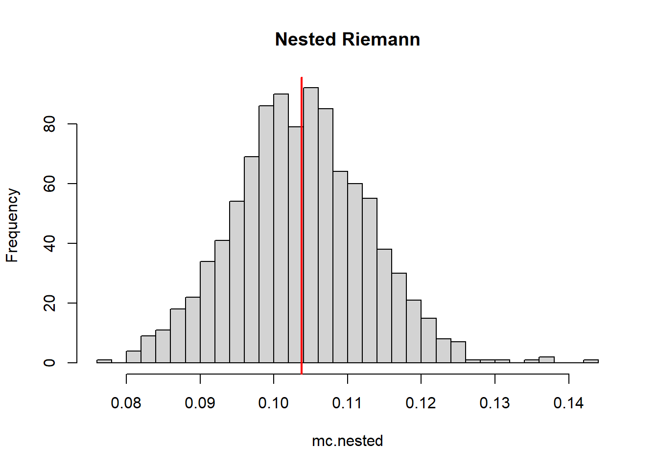

hist(mc.nested.rect, breaks = 30, main = "Nested Rectangular")
abline(v=trueZ,col="red",lwd=2)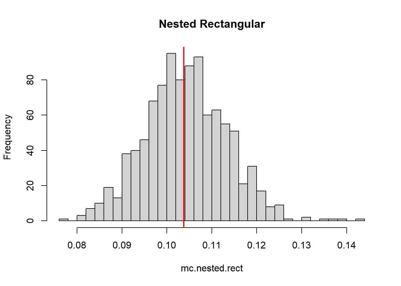

Comparison

Performance table

### Comparison table

## Numerical 

mean.qis <- mean(mc.qis); 
mean.naive <- mean(mc.naive)
median.qis <- median(mc.qis); median.naive <- median(mc.naive)
mape.qis <- median(abs((mc.qis)-(trueZ))/(trueZ))
mape.naive <- median(abs(((mc.naive)-(trueZ))/(trueZ)))
rmse.qis <- sqrt((mean((mc.qis-trueZ)^2)))
rmse.naive <- sqrt((mean((mc.naive-trueZ)^2)))

mean.nested <- mean(mc.nested); 
mean.nested.rect <- mean(mc.nested.rect)
median.nested <- median(mc.nested); median.nested.rect <- median(mc.nested.rect)
mape.nested <- median(abs((mc.nested)-(trueZ))/(trueZ))
mape.nested.rect <- median(abs(((mc.nested.rect)-(trueZ))/(trueZ)))
rmse.nested <- sqrt((mean((mc.nested-trueZ)^2)))
rmse.nested.rect <- sqrt((mean((mc.nested.rect-trueZ)^2)))

perf <- rbind((cbind(mean.qis,mean.naive,mean.nested,mean.nested.rect)),
              # (cbind(median.qis,median.naive)),
              (cbind(mape.qis, mape.naive,mape.nested, mape.nested.rect)),
              (cbind(rmse.qis,rmse.naive, rmse.nested, rmse.nested.rect)))

colnames(perf) <- c("QIS", "Naive", "Nested-Rect", "Nested-Riemann"); 
row.names(perf) <- c("Mean", "MAPE", "RMSE")

library(kableExtra)
kable(perf, format = "html") %>%
  kable_styling()

	QIS	Naive	Nested-Rect	Nested-Riemann
Mean	0.1039080	0.1038586	0.1036941	0.1042129
MAPE	0.0214313	0.0730794	0.0583801	0.0583841
RMSE	0.0035507	0.0115004	0.0090859	0.0091414

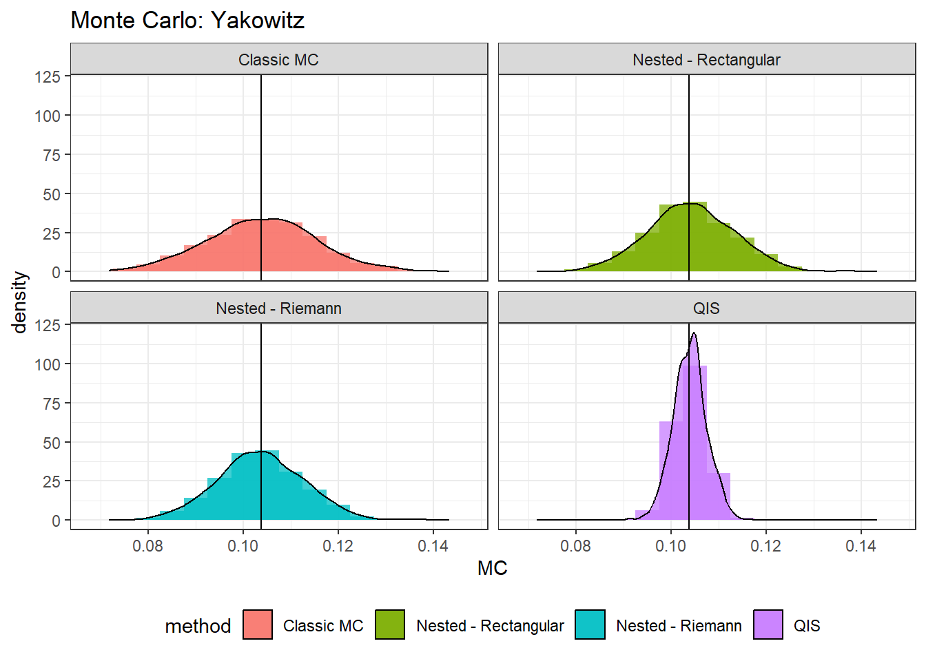
Visual comparison

library(ggplot2)
mc.data = rbind(data.frame(MC = mc.qis, method = "QIS"),
                data.frame(MC = mc.nested.rect, method = "Nested - Rectangular"),
                data.frame(MC = mc.nested, method = "Nested - Riemann"),
                 data.frame(MC = mc.naive, method = "Classic MC"))

(norm.plt <- ggplot(mc.data, aes(MC, fill = method)) + 
    geom_histogram(alpha=0.75,binwidth = 0.005, position="identity",aes(y = ..density..))+
    geom_density(alpha=0.75,adjust = 1, stat="density",position="identity",aes(y = ..density..))+
    geom_vline(xintercept=trueZ)+ #coord_flip()+
    facet_wrap(vars(method), ncol = 2, scales = "fixed") + 
    ggtitle(paste0("Monte Carlo: Yakowitz"))+
    theme_bw()+
    theme(legend.position = "bottom")
)